bands-inspect¶

This is a tool to create, compare and plot bandstructures of materials.

Installation
Tutorial

Installation ¶

You can install this tool with pip:

pip install bands-inspect

Tutorial ¶

The following tutorial illustrates some examples of the most important functionality in the bands-inspect library.

Defining k-points ¶

The bands-inspect code defines different ways of defining a set of k-points:

Explicit k-points ¶

First, k-points can be given explicitly as a nested list:

In [1]: import bands_inspect as bi
   ...: import numpy as np
   ...: 

In [2]: kpts_explicit = bi.kpoints.KpointsExplicit(
   ...:     [[0, x, x] for x in np.linspace(0, 1, 6)]
   ...: )
   ...: 
Out[2]: 
namespace(kpoints=array([[0. , 0. , 0. ],
                         [0. , 0.2, 0.2],
                         [0. , 0.4, 0.4],
                         [0. , 0.6, 0.6],
                         [0. , 0.8, 0.8],
                         [0. , 1. , 1. ]]))

K-point mesh ¶

Second, an even mesh of k-points can be generated by giving the size of the mesh. A constant offset for the mesh points can also be set:

In [3]: kpts_mesh = bi.kpoints.KpointsMesh([2, 3, 2])
Out[3]: namespace(mesh=(2, 3, 2), offset=array([0, 0, 0]))

In [4]: kpts_mesh_offset = bi.kpoints.KpointsMesh([2, 3, 2], offset=[0.1, 0, -0.1])
Out[4]: namespace(mesh=(2, 3, 2), offset=array([ 0.1,  0. , -0.1]))

To check the generated k-points, all such k-point classes have a property kpoints_explicit which contains the explicit list of points:

In [5]: kpts_mesh.kpoints_explicit
Out[5]: 
array([[0.        , 0.        , 0.        ],
       [0.        , 0.        , 0.5       ],
       [0.        , 0.33333333, 0.        ],
       [0.        , 0.33333333, 0.5       ],
       [0.        , 0.66666667, 0.        ],
       [0.        , 0.66666667, 0.5       ],
       [0.5       , 0.        , 0.        ],
       [0.5       , 0.        , 0.5       ],
       [0.5       , 0.33333333, 0.        ],
       [0.5       , 0.33333333, 0.5       ],
       [0.5       , 0.66666667, 0.        ],
       [0.5       , 0.66666667, 0.5       ]])

In [6]: kpts_mesh_offset.kpoints_explicit
Out[6]: 
array([[0.1       , 0.        , 0.9       ],
       [0.1       , 0.        , 0.4       ],
       [0.1       , 0.33333333, 0.9       ],
       [0.1       , 0.33333333, 0.4       ],
       [0.1       , 0.66666667, 0.9       ],
       [0.1       , 0.66666667, 0.4       ],
       [0.6       , 0.        , 0.9       ],
       [0.6       , 0.        , 0.4       ],
       [0.6       , 0.33333333, 0.9       ],
       [0.6       , 0.33333333, 0.4       ],
       [0.6       , 0.66666667, 0.9       ],
       [0.6       , 0.66666667, 0.4       ]])

Finally, the k-points can be described as a set of special points, and one or more paths going between these paths. The paths are given as a nested list of identifiers, while the points itself are given as a dictionary mapping these identifiers to the corresponding coordinate:

In [7]: kpts_path = bi.kpoints.KpointsPath(
   ...:     paths=[['L', 'X', '$\Gamma$'], ['L', '$\Gamma$']],
   ...:     special_points={
   ...:         '$\Gamma$': [0, 0, 0],
   ...:         'X': [0, 0.5, 0.5],
   ...:         'L': [0.5, 0.5, 0.5],
   ...:     }
   ...: )
   ...: 
Out[7]: <bands_inspect.kpoints._path.KpointsPath at 0x7f8b5b07a588>

In [8]: kpts_path.kpoints_explicit
Out[8]: 
array([[5.00000000e-01, 5.00000000e-01, 5.00000000e-01],
       [4.99840866e-01, 5.00000000e-01, 5.00000000e-01],
       [4.99681731e-01, 5.00000000e-01, 5.00000000e-01],
       ...,
       [1.83789745e-04, 1.83789745e-04, 1.83789745e-04],
       [9.18948723e-05, 9.18948723e-05, 9.18948723e-05],
       [0.00000000e+00, 0.00000000e+00, 0.00000000e+00]])

Note that this produces k-points which are equally spaced in reduced coordinates, not in the more physical Cartesian coordinates. To remedy this, a unit cell can be given. Furthermore, the maximum distance between any two k-points can be controlled by a parameter kpoint_distance:

In [9]: a = 3.2395
   ...: kpts_path_with_uc = bi.kpoints.KpointsPath(
   ...:     paths=[['L', 'X', '$\Gamma$'], ['L', '$\Gamma$']],
   ...:     special_points={
   ...:         '$\Gamma$': [0, 0, 0],
   ...:         'X': [0, 0.5, 0.5],
   ...:         'L': [0.5, 0.5, 0.5],
   ...:     },
   ...:     kpoint_distance=0.1,
   ...:     unit_cell=[[0, a, a], [a, 0, a], [a, a, 0]]
   ...: )
   ...: 
Out[9]: <bands_inspect.kpoints._path.KpointsPath at 0x7f8b5b07abe0>

In [10]: kpts_path_with_uc.kpoints_explicit
Out[10]: 
array([[0.5   , 0.5   , 0.5   ],
       [0.4375, 0.5   , 0.5   ],
       [0.375 , 0.5   , 0.5   ],
       [0.3125, 0.5   , 0.5   ],
       [0.25  , 0.5   , 0.5   ],
       [0.1875, 0.5   , 0.5   ],
       [0.125 , 0.5   , 0.5   ],
       [0.0625, 0.5   , 0.5   ],
       [0.    , 0.5   , 0.5   ],
       [0.    , 0.45  , 0.45  ],
       [0.    , 0.4   , 0.4   ],
       [0.    , 0.35  , 0.35  ],
       [0.    , 0.3   , 0.3   ],
       [0.    , 0.25  , 0.25  ],
       [0.    , 0.2   , 0.2   ],
       [0.    , 0.15  , 0.15  ],
       [0.    , 0.1   , 0.1   ],
       [0.    , 0.05  , 0.05  ],
       [0.    , 0.    , 0.    ],
       [0.5   , 0.5   , 0.5   ],
       [0.4375, 0.4375, 0.4375],
       [0.375 , 0.375 , 0.375 ],
       [0.3125, 0.3125, 0.3125],
       [0.25  , 0.25  , 0.25  ],
       [0.1875, 0.1875, 0.1875],
       [0.125 , 0.125 , 0.125 ],
       [0.0625, 0.0625, 0.0625],
       [0.    , 0.    , 0.    ]])

Creating eigenvalue objects ¶

The data container used in the bands-inspect code is the EigenvalsData class. It contains a list of k-points (either given explicitly or as a k-points object), and a corresponding array of eigenvalues:

In [11]: ev_explicit = bi.eigenvals.EigenvalsData(
   ....:     kpoints=[[0, 0, 0], [0.1, 0.1, 0.1]],
   ....:     eigenvals=[[-0.124, 0.001123, 0.51234], [-0.132, 0.013, 0.412]]
   ....: )
   ....: 
Out[11]: 
namespace(kpoints=namespace(kpoints=array([[0. , 0. , 0. ],
                                           [0.1, 0.1, 0.1]])),
          eigenvals=array([[-0.124   ,  0.001123,  0.51234 ],
                           [-0.132   ,  0.013   ,  0.412   ]]))

When a Python function that calculated the eigenvalues at a given k-point is known, the from_eigenval_function() method can be used to conveniently build such an EigenvalsData object. For example, if we have a tight-binding model from the TBmodels code:

In [12]: import tbmodels
   ....: model = tbmodels.io.load(SAMPLES_DIR / 'InSb.hdf5');
   ....: 

In [13]: ev_from_function = bi.eigenvals.EigenvalsData.from_eigenval_function(
   ....:     kpoints=kpts_path_with_uc,
   ....:     eigenval_function=model.eigenval
   ....: );
   ....: 

Plotting ¶

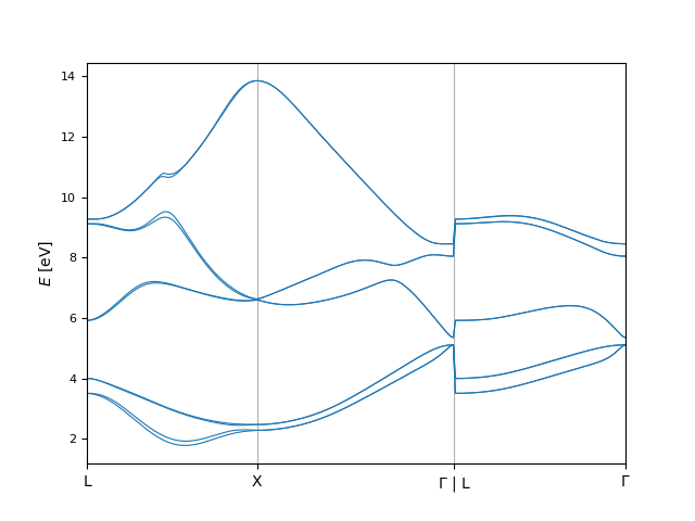
Having created the EigenvalsData instance, we can plot the bandstructure with the plot.eigenvals() function:

In [14]: bi.plot.eigenvals(ev_from_function);

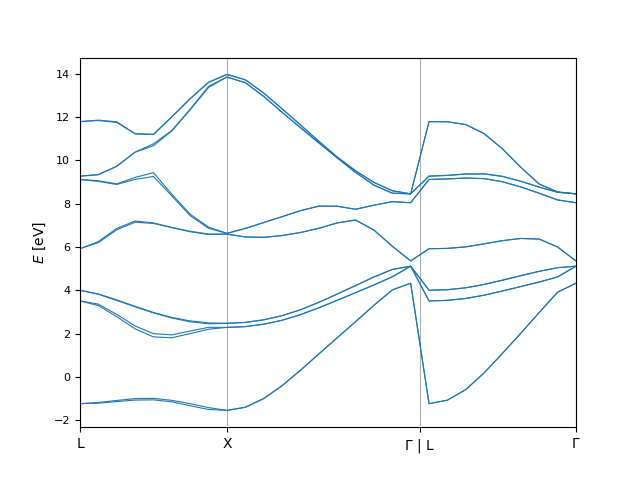
Of course, we can create a finer version of this plot by repeating the same procedure with a smaller kpoint_distance:

In [15]: kpt_fine = bi.kpoints.KpointsPath(
   ....:     paths=[['L', 'X', '$\Gamma$'], ['L', '$\Gamma$']],
   ....:     special_points={
   ....:         '$\Gamma$': [0, 0, 0],
   ....:         'X': [0, 0.5, 0.5],
   ....:         'L': [0.5, 0.5, 0.5],
   ....:     },
   ....:     kpoint_distance=0.01,
   ....:     unit_cell=[[0, a, a], [a, 0, a], [a, a, 0]]
   ....: )
   ....: ev_fine = bi.eigenvals.EigenvalsData.from_eigenval_function(
   ....:     kpoints=kpt_fine,
   ....:     eigenval_function=model.eigenval
   ....: )
   ....: bi.plot.eigenvals(ev_fine);
   ....: 

Saving objects ¶

K-point and eigenvalue objects (and combinations of such objects) can be saved in the HDF5 format using the io.save() function, and loaded using io.load():

In [16]: import tempfile
   ....: with tempfile.NamedTemporaryFile() as tf:
   ....:     bi.io.save([kpt_fine, ev_explicit], tf.name)
   ....:     kpt_res, ev_res = bi.io.load(tf.name)
   ....: 

In [17]: kpt_res
Out[17]: <bands_inspect.kpoints._path.KpointsPath at 0x7f8b59c69358>

In [18]: ev_res
Out[18]: 
namespace(kpoints=namespace(kpoints=array([[0. , 0. , 0. ],
                                           [0.1, 0.1, 0.1]])),
          eigenvals=array([[-0.124   ,  0.001123,  0.51234 ],
                           [-0.132   ,  0.013   ,  0.412   ]]))

Band difference ¶

The bands-inspect library also defines functionality for comparing bandstructures. Specifically, it allows for computing the difference between two sets of eigenvalues with equal k-points. This is implemented in the compare.difference.calculate() function. By default, it computes the average difference

\[\Delta = \frac{1}{M}\frac{1}{N_{\mathbf{k}}} \sum\limits_{i=1}^{M} \sum\limits_{\mathbf{k}} \left| \varepsilon_{i, \mathbf{k}} - \varepsilon_{i, \mathbf{k}}' \right|,\]

where \(i\) is the band index.

In [19]: ev_fine_modified = bi.eigenvals.EigenvalsData.from_eigenval_function(
   ....:     kpoints=kpt_fine,
   ....:     eigenval_function=lambda k: model.eigenval(k) * 1.1
   ....: )
   ....: 
   ....: bi.compare.difference.calculate(ev_fine, ev_fine_modified)
   ....: 
Out[19]: 0.641595461618997

Since not all energy ranges or k-points are always equally important when comparing band-structures, it is also possible to define weights for the k-points and energies. The computed difference then becomes

\[\Delta = \frac{\sum\limits_{i, \mathbf{k}} \left| \varepsilon_{i, \mathbf{k}} - \varepsilon_{i, \mathbf{k}}' \right| w_1(\mathbf{k}) w_2(\varepsilon_{i, \mathbf{k}}, \varepsilon_{i, \mathbf{k}}')}{\sum\limits_{i, \mathbf{k}} w_1(\mathbf{k}) w_2(\varepsilon_{i, \mathbf{k}}, \varepsilon_{i, \mathbf{k}}')}\]

The weights are given as functions which take all k-points / energies and return a corresponding array of weights. For the energies, one can choose whether the function is supplied with the average of the two values (if symmetric_eigenval_weights=True) or only the first value. This latter option is useful if many different band structures need to be compared against a single reference, to ensure that the weights are always the same.

For example, let us calculate the difference where only the first \(100\) k-points and energies above \(6~\text{eV}\) are taken into account:

In [20]: def kpt_weight(kpts):
   ....:     res = np.zeros(np.array(kpts).shape[0])
   ....:     res[:100] = 1
   ....:     return res
   ....: 

In [21]: def ev_weight(energy):
   ....:     return np.array(energy > 6, dtype=int)
   ....: 

In [22]: bi.compare.difference.calculate(
   ....:     ev_fine,
   ....:     ev_fine_modified,
   ....:     weight_kpoint=kpt_weight,
   ....:     weight_eigenval=ev_weight,
   ....: )
   ....: 
Out[22]: 0.9713096623784362

Furthermore, the function used to calculate the average can also be defined by the user. By default, np.average is used.

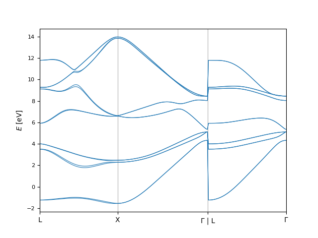
Slicing bands ¶

Often, band structures with different number of bands need to be compared. To do this, the bands need to first be reduced such that their band indices match. This can be done using the slice_bands() method of EigenvalsData objects. In the following example, we reduce the previously seen bandstructure of InSb by cutting the two lowest and highest bands.

In [23]: ev_sliced = ev_fine.slice_bands(range(2, 12))
   ....: bi.plot.eigenvals(ev_sliced)
   ....: 
Out[23]: <Figure size 640x480 with 1 Axes>